How to learn RF Bandpass filter?

Methods for Learning RF Bandpass Filters
RF Bandpass Filter (BPF) plays a crucial role in wireless communications, radar systems, and RF circuits. Its primary function is to allow signals within a specific frequency band to pass through and suppress other unnecessary frequencies. For amateur RF engineers and students, learning about BPF requires understanding of fundamental principles, frequency characteristics, tuning techniques, testing methods, and various types of applications. Below are several key focus areas for effective learning:
Step 1: Understand the basic principles of RF filters
The first step to learning BPF is to understand its operating principle. Bandpass filters mainly selects a specific frequency range through LC resonant circuit, mechanical resonance or acoustic wave technology. Learning the relationship between parameters such as Q value (quality factor), center frequency, bandwidth, insertion loss and out-of-band rejection will help you understand how to set the appropriate filter for different product environments and application requirements.
Step 2: Learn the frequency response curve of BPF
Frequency response curves are important tools for evaluating BPF performance. Common indicators include S21 (transmission characteristics) and S11 (reflection characteristics). By understanding the shape of these curves—including the filter’s passband range, bandwidth, cutoff frequencies, and attenuation behavior—engineers can use the response graph to quickly determine whether a filter meets the design requirements of a given product.
Step 3: Learn how to tune and set a BPF
BPF’s frequency characteristics can be modified by adjusting its internal structure setting.For example, Cavity filter and Helical filter can change the frequency and performance parameters by adjusting the tuning screw and adjusting the coil spacing. By physically tuning the filter, we can have a deeper understanding of the Filter operation, thereby enhancing their design capabilities and practical RF engineering skills.
Step 4: Learn how to measure and verify BPF performance
A filter must be tested using a network analyzer (NA) to accurately display its frequency response curve, which is essential for evaluating its performance. Therefore, learning how to correctly operate the network analyzer (NA) and use the network analyzer (NA) to accurately output the filter parameter performance is an essential skill for RF engineers and related users.
Step 5: Explore different types of BPFs and compare their applications
There are many types of BPF. RF filters made based on different technologies can be applied to different product applications, each with its own advantages and disadvantages. Common types include Cavity, Helical, Dielectric Resonator (DR), and SAW (Surface Acoustic Wave) filters. Understanding the strengths and limitations of these technologies will help you choose the most suitable filter type to meet various design requirements.
Through these five learning steps, you can gradually build up your understanding of RF Bandpass Filter and apply that knowledge to real-world RF design and tuning. Continuous learning and practice will help you become more proficient in the field of RF engineering!

Basic principles of RF filters
The core function of RF filter is to selectively allow signals within a certain frequency range to pass through—while suppressing signals at other frequencies—by using LC resonant circuits, mechanical resonance, or acoustic wave technologies. Its performance is primarily determined by several key parameters: center frequency, bandwidth, insertion loss, and out-of-band rejection. These parameters are interrelated and have a mutual impact on one another.
Center frequency determines the middle point of the filter passband. For example, a filter used for 2.4GHz Wi-Fi is typically set with a center frequency at 2.45GHz, allowing Wi-Fi signals to pass effectively while suppressing interference from other frequency bands. Bandwidth determines the passable frequency range. A wider bandwidth allows more signals to pass but may reduce the ability to suppress adjacent out-of-band signals. On the other hand, a narrower bandwidth improves frequency selectivity but may result in higher insertion loss.
Insertion loss represents to the reduction in signal power as it passes through the filter. When the bandwidth becomes narrower, it can show better suppression ability, but at the same time it will cause higher insertion loss, so it is necessary to make a trade-off between coverage and energy loss during design. In addition, out-of-band suppression is the filter's ability to isolate signals outside the passband. Strong out-of-band suppression can quickly and effectively filter out unnecessary interference, but it usually increases the complexity and difficulty of the design, and insertion loss needs to be considered together.
The relationship between these parameters determines the effectiveness of the filter. For example, improving out-of-band suppression usually requires adding circuit stages, which may lead to higher insertion loss; widening bandwidth may reduce out-of-band suppression, etc. Therefore, when designing a filter, it is essential to balance these parameters according to the specific application requirements in order to achieve optimal frequency selectivity.

Frequency response curve of BPF
Frequency response curve describes how signals are transmitted and reflected at different frequency point, typically analyzed using S-parameters (S11 and S21). S11 represents the reflection coefficient (return loss), indicating how much of the input signal is reflected back. S21 represents the transmission coefficient (insertion loss), showing the amount of signal attenuation after passing through the filter.
On the frequency response curve, the center frequency (f₀) is the middle point of the passband, corresponding to the highest point of the S21 curve, indicating that the signal of this frequency can pass through the filter most effectively. The bandwidth is determined by the -3dB point, and sometimes the -1dB point , is used to represent the range in which the signal can be effectively transmitted. The steeper the slope of the S21 curve, the greater the filter's ability to isolate signals, effectively excluding interfering signals outside the passband from the response curve.
Insertion Loss (IL) is represented on the S21 curve as the attenuation value at the center frequency. It is typically measured in decibels (dB), with smaller values indicating less signal energy loss. In other words, the lower the insertion loss, the more efficiently the signal passes through the filter at its intended frequency.
On the other hand, out-of-band attenuation refers to the filter's ability to suppress signals outside the passband, starting from the center frequency and extending into the stopband. The filter's suppression energy is strongest at the center frequency, and the farther away from the center frequency, the weaker the energy. The effectiveness of out-of-band attenuation can be evaluated in two key aspects. First, the closer to the center frequency, the higher the attenuation value can be, indicating that the filter's energy can be fully concentrated within the target frequency band to work, and the energy is not lost. Second, the attenuation value is not only high, but also continue to extend to very far frequencies, indicating that the filter's coverage energy is very good and can fully suppress the interference of second and third harmonics.
On a frequency response curve, second harmonics may appear, typically occurring at twice the center frequency. For example, if the center frequency (f₀) is 1 GHz, an additional response may appear near 2 GHz. This can result from nonlinear effects or parasitic responses and may impact overall system performance. Therefore, when analyzing the filter frequency response curve, it is necessary to pay attention to whether the second harmonic will occur, and pre-suppress these unnecessary harmonics during design to ensure stable signal quality.

How to tune and set a BPF
When adjusting a Bandpass Filter (BPF), different methods need to be adopted according to the type of filter to ensure that its center frequency, bandwidth and attenuation characteristics meet the design requirements.
Cavity filters are typically used in high-power and high-Q applications. When adjusting, the resonant frequency can be adjusted by modifying the tuning screws inside the cavity, while the bandwidth can be altered by changing the coupling structure. Additionally, adjustments to the spacing between cavities can influence performance parameters and out-of-band suppression. Under the structural tuning method, although fine-tuning can still be performed through screws after the production procedure is completed, the adjusting operation requires mechanical tools and equipment, making he adjustment operation is more difficult and complex for general users.
DR Filter (Dielectric Resonance Filter) uses high dielectric constant materials to form resonance and is suitable for microwave frequency bands. Due to the limitation of material characteristics, the filter parameters must be defined during the simulation and design phase, and achieved through precise manufacturing. As a result, the ability to fine-tune the filter after production is limited, and adjustments typically require a complete redesign and remanufacturing process.
SAW Filter (Surface Acoustic Wave Filter) uses acoustic wave transmission on piezoelectric materials to achieve filtering functions and is widely used in mobile phones and wireless communication devices. The frequency response of SAW filters is fixed during the manufacturing process. The center frequency and bandwidth are determined by the process. Therefore, once the production is completed, it cannot be manually fine-tuned. The manufacturing parameters must be precisely controlled during the design stage to ensure that they meet the requirements.
Helical Filters are primarily used in VHF/UHF bands, using spiral inductors to generate resonance. Adjustments methods include changing the length or spacing of the coils to modify the center frequency and bandwidth, or moving the height of the screws to affect the filter parameters. This type of filter usually allows a certain degree of manual fine-tuning after production, and the adjustment frequency range can reach to approximately 3-10MHz. This makes them suitable for amateur RF engineers and students, who can achieve precise frequency tuning through repeated hands-on practice.
By actually adjusting the frequency response curve of the filter, learners can have a deeper understanding of how the filter operates and how its performance changes. This hands-on experience enhances practical skills and better equips engineers to design products that more closely meet real-world requirements in the future.

How to measure and verify BPF performance
When using a network analyzer (NA) to measure the frequency response curve of RF filter, it is necessary to ensure the correct connection method, the use of the test fixture, and accurate calibration to obtain reliable measurement results.
First, choose the appropriate test fixture, especially for filters without connectors—such as SAW or DR filters mounted on a PCB—which may require dedicated clamps or probes to ensure proper connection while minimizing additional insertion loss and reflection. For filters equipped with SMA, N-type, or 2.92mm connectors, standard RF cables can be used for direct connection. Connect the input end (Port 1) of the filter to the output port (Port 1) of the VNA, and the output end (Port 2) to the input port (Port 2) of the VNA to measure S21 (transmission coefficient) and S11 (reflection coefficient).
Before measurement, of course, calibration must be performed. Calibration refers to the process of compensating for measurement errors in equipment such as a Network Analyzer (NA), in order to eliminate the influence of connecting wires, connectors, test fixtures and the equipment itself. This ensures that the measurement results are accurate and reliable. Since the signal must pass through the test cable and connector when the VNA performs S parameter measurement, these components will produce additional insertion loss, reflection and phase error, so calibration is required before testing to compensate for these influences.
Common calibration methods include 1-port calibration and 2-port calibration. 1-port calibration uses the standards of Open, Short and Load to correct the S11 test results, while 2-port calibration uses additional Through standards to ensure the accuracy of S21 measurements. Furthermore, when using test fixtures, it is recommended to perform de-embedding to compensate for the influence of the fixture on the measurement results, ensuring that the data reflects the true performance of the device under test.
After calibration is completed, set the scanning frequency range (Start/Stop Frequency), resolution bandwidth (RBW) and output power to ensure appropriate test conditions. Finally, perform the frequency sweep to obtain the frequency response curve of the filter, and further analyze the center frequency, bandwidth, insertion loss and out-of-band suppression to ensure that the filter performance meets the required specifications.

Feature of different RF Bandpass Filter types
Bandpass filters (BPFs) can be categorized into Cavity Filters, Helical Filters, Dielectric Resonator Filters (DR Filters), and Surface Acoustic Wave (SAW) Filters, depending on their design methods and materials. Each type differs in terms of structure, appearance, performance, and application.
1. Cavity Bandpass Filter
Structure and Appearance:
Uses a metal cavity and tuning screws to create resonance. Typically features a box-shaped metal housing with relatively large dimensions. Connected via SMA or N-type connectors.
Performance:
High Q value, low insertion loss, suitable for high power applications, but large volume. Performance can be fine-tuned again through mechanical equipment.
Frequency Range:
300 MHz to above 80 GHz.
Applications:
Wireless communication base stations, radar systems, and military equipment.
2. Helical Bandpass Filter
Structure and Appearance:
Resonance is formed by coupling spiral inductors and capacitors. These filters are relatively compact and typically housed in cylindrical or rectangular metal enclosures. They are connected via PINs and directly soldered onto PCB.
Performance:
Moderate Q value, low insertion loss, large flexibility in parameter design, and filter performance can be fine-tuned at any time through simple tools.
Frequency Range:
VHF/UHF bands (30 MHz to 2.6 GHz).
Applications:
Radio communications, television transmitters, and mobile communications.
3. Dielectric Resonator Bandpass Filter (DR Filter)
Structural appearance:
Use ceramic materials with high dielectric constant as resonators. Usually a small rectangular structure with ceramic resonator blocks inside. Connected via SMD interfaces and directly soldered onto PCBs.
Performance:
High Q value, small size, low insertion loss, high temperature adaptability, and suitable operating temperature specifications can be designed according to different temperature environment requirements. Performance fine-tuning cannot be performed again.
Frequency Range:
From 300 MHz to 6 GHz.
Applications:
Microwave communication, 5G equipment, and satellite communication.
4.SAW Bandpas Filter (Surface Acoustic Wave Filter)
Structure and Appearance:
Implements filtering through acoustic wave propagation on piezoelectric materials. Extremely compact in size and well-suited for mass production. Connected via SMD (Surface Mount Device) packaging and directly soldered onto PCB.
Performance:
small size, low cost, suitable for high-density circuits, but low Q value and high insertion loss. Performance cannot be fine-tuned again.
Frequency Range:
From 300 MHz to 6 GHz.
Applications:
Mobile phones, Wi-Fi, GPS, and RF front-end modules.
Different types of BPFs have their own advantages in terms of performance, size, and application areas. To achieve the most suitable design outcome, it is important to select the appropriate filter type based on the product's functional objectives and design constraints.

Learning RF Filter principles with RF Education Tool Kit
Learning RF filters requires not only theoretical knowledge, but also hands-on experience to fully understand the characteristics and adjusting skills. With RF Education Tool Kit, students and amateur RF engineers can measure and adjust filters themselves, gaining a more comprehensive understanding of how filters work.
Learning how to actually measure filters is an important step in learning RF technology. RF Education Tool Kit allows learners to touch and operate filters with their own hands, and truly feel the physical structure and working method of electronic components. By directly interacting with different types of filters—such as Cavity, Helical, or SAW—learners gain a clear understanding of the design architecture and operating principles of each type. They can also use a network analyzer (NA) to measure the reflection coefficient (S11) and transmission coefficient (S21) of the filter, observing how the filter affects signal reception and transmission. This practical experience not only reinforces theoretical knowledge but also helps learners intuitively grasp the real-world role of filters in RF systems.

Secondly, learn how to connect the filter to the network analyzer. In the filter learning, it is very important to use RF Education Tool Kit to learn the correct measurement method. RF Education Tool Kit is typically equipped with standard SMA or N-type connectors, along with test fixtures PCB, allowing learners to correctly connect filters to a network analyzer (NA). In addition, learners can practice the calibration procedure, gaining a deeper understanding of how to eliminate errors caused by test cables or equipment, thereby improving measurement accuracy. In addition, learners can also learn to identify and deal with various abnormal situations that may occur during the measurement process.
Finally, RF Education Tool Kit allows learners to physically adjust the filter and observe the performance curve changes in the filter, which is a key experience to develop practical skills. Filters (such as Cavity or Helical) allow manual tuning of the filter parameters and frequency response curve. Learners can rotate tuning screws to modify component values and directly observe how changes affect the center frequency, bandwidth, and insertion loss. This real-time interaction helps deepen the understanding of how frequency response curves can be adjusted and optimized.

Helical RF BPF Learning Tool Kit from Temwell
Temwell develops and supplies Helical RF BPF Learning Tool Kit to help learners gain a deeper understanding of the design, testing and application of RF Bandpass Filters. When studying RF technology, many learners often face challenges such as lack of suitable practical tools, difficulty in obtaining high-quality filters, and expensive testing equipment. Therefore, Temwell provides professional-grade Helical BPFs, dedicated PCB, and SMA/N connectors to create a complete learning solution to address these pain points.
The toolkit includes the following components:
1.RF Helical BPF x 2pcs—— Includes two Helical Bandpass Filters, with customizable specifications such as center frequency, bandwidth, and ejection value based on user requirements. This allows learners to test filters with specific frequency band and characteristics, gaining a deeper understanding of their applications. RF Filters can be selected directly from 3000 standard items online in Temwell website.
2.Layout PCB x 2pcs —— Includes two PCB layouts designed specifically for Helical BPF, which is convenient for learners to practice soldering and circuit assembly, and learn how to integrate the filter into the RF module effectively.
3. SMA-Female Connector x 2 pcs (Optional N-Female) —SMA-Female connector is provided by default, which can be replaced with N-Female to support the interface requirements of different devices and ensure the flexibility and compatibility of the test.

Through Temwell Helical RF BPF Learning Tool Kit, learners can personally design specification parameters, assemble and hands-on test filters, master core technologies such as frequency response, bandwidth tuning, and insertion loss measurement, and learn how to properly connect and calibrate a network analyzer (NA). With 30 years of professional experience in RF filters, Temwell ensures that each component meets industry standards, allowing learners to get the best learning experience and a strong foundation to confidently enter the RF communication field!
Whether you are a student, RF engineer or radio enthusiast, this toolkit can help you get started easily and quickly enhance your RF design and testing capabilities! Experience it now and start your RF learning journey! 🚀
Feel free to contact us and get free consultation services so that we can provide you with the best solution.
Subscribe to us on Facebook for the latest product news.