Ultra-Wideband Cavity Bandpass Filter Impedance Matching Strategies

2026-09-14

Abstract

Ultra-wideband (UWB) technology plays a critical role in modern wireless communications, radar, electronic warfare, and instrumentation systems. One of its core challenges is maintaining uniform, low-loss impedance matching across an extremely wide frequency band. From the viewpoint of a microwave engineer, this paper systematically examines the impedance-matching principles and design strategies for UWB cavity bandpass filters, covering the theoretical limit (the Bode–Fano criterion), multi-section Chebyshev matching networks, tapered-line designs, and an analysis of real Temwell product specifications, and finally provides system-integration verification methods and selection guidelines.

Keywords: impedance matching, bandwidth, Bode–Fano criterion, Chebyshev multi-section matching, Klopfenstein taper, VSWR, ultra-wideband cavity bandpass filter, TEMWELL.

1. Introduction: The Rise of UWB Applications and the Matching Challenge

1.1 Background of UWB Technology

UWB technology has steadily become an indispensable element of modern communication architectures since the FCC opened the commercial band (3.1–10.6 GHz) in 2002. UWB is defined as an operating band with a fractional bandwidth (FBW) exceeding 163%, or a frequency ratio (f_H／f_L) greater than 10:1.^[1]

UWB technology is widely deployed in:

Radar and sensing: through-wall radar, ground-penetrating survey, medical imaging.
Wideband receivers: ELINT and SIGINT systems.
Millimeter-wave communications: 5G/6G infrastructure, satellite links.^[2]
Test instrumentation: network analyzers, spectrum analyzers.
Electronic warfare: fast frequency hopping, wideband jamming.

1.2 The Core Matching Challenge

The most fundamental challenge for a UWB bandpass filter is how to simultaneously maintain low insertion loss and uniform impedance matching across a band spanning several octaves. The wider the band, the harder it is to optimize impedance at every frequency at once — a problem fundamentally constrained by the Bode–Fano criterion.^[3]

Temwell's UWB cavity bandpass filter line spans 500 MHz to 28 GHz, with some models offering passbands of several GHz, reflecting the state of the art in modern UWB design.^[2]

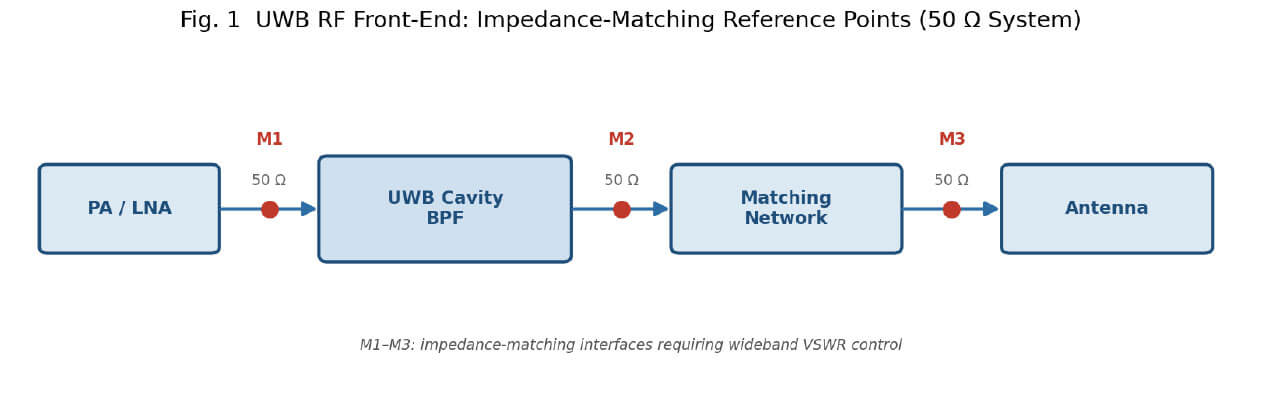
Fig. 1 UWB RF front-end impedance-matching reference points (50 Ω system): M1–M3 are interfaces requiring wideband VSWR control.

2. Matching Fundamentals: The 50 Ω Standard and Consequences of Mismatch

2.1 The 50 Ω System Standard

Modern RF/microwave systems universally adopt 50 Ω, a compromise between maximum power capacity (~30 Ω) and minimum attenuation (~77 Ω) of a coaxial line. All RF components are designed around 50 Ω for maximum power-transfer efficiency.^[3]

Γ = ( Z_L − Z₀ ) / ( Z_L + Z₀ )

where Z_L is the load impedance and Z₀ the system characteristic impedance (50 Ω). For a perfect match Γ = 0; the worse the mismatch, the closer |Γ| approaches 1. The standing-wave ratio is:

VSWR = ( 1 + |Γ| ) / ( 1 − |Γ| )

2.2 Practical Consequences of Poor Matching

Table 1. Consequences of poor impedance matching

Problem	Physical Mechanism	System Impact
Signal reflection	Incident wave partly reflected	Power loss, standing waves
Higher insertion loss	Return loss degrades	Lower effective output power
Power mismatch loss	Max power not delivered	Worse link budget
Group-delay distortion	Non-uniform phase velocity	Waveform distortion, timing skew
Amplifier instability	Reflection returns to amp input	Oscillation / gain ripple

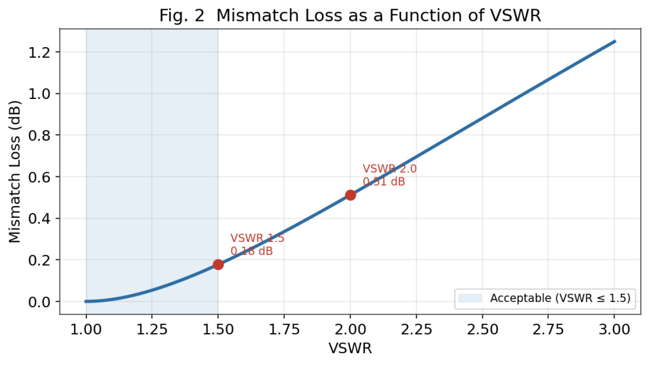
In practice, VSWR ≤ 1.5:1 (RL ≥ 14 dB) is regarded as acceptable matching quality.^[4][2]

L_mismatch (dB) = −10 · log₁₀( 1 − |Γ|² )

Fig. 2 Mismatch loss as a function of VSWR; VSWR ≤ 1.5 corresponds to < 0.18 dB loss.

3. Why Wideband Matching Is Hard: The Physical Reasons

3.1 The Bode–Fano Criterion

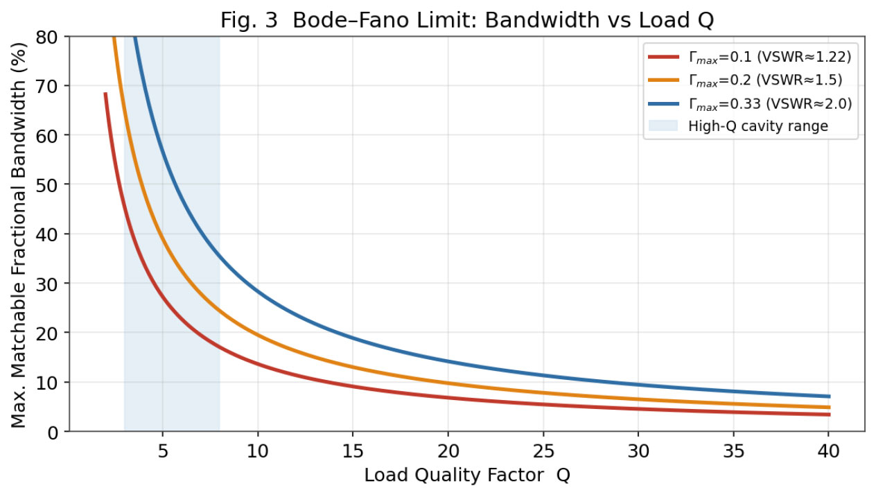
The root cause of UWB matching difficulty is the Bode–Fano criterion, an information-theoretic limit setting the maximum matching bandwidth achievable by any passive, linear, time-invariant network.^[5][3] For a parallel-RC load:

∫₀^∞ ln( 1 / |Γ(ω)| ) dω ≤ π / (R·C)

For a general load, using the quality factor Q:

( BW / ω₀ ) · ln( 1 / Γ_avg ) ≤ π / Q

This reveals three constraints: (1) higher Q narrows the matchable bandwidth; (2) match quality and bandwidth cannot both be maximized; (3) perfect matching over a finite band is impossible for a reactive load.

Fig. 3 Bode–Fano limit: matchable bandwidth vs. load Q; the high-Q cavity region (shaded) is bandwidth-limited.

3.2 Practical Meaning

For a load with Q = 10 and Γ_max = 0.3 (VSWR ≈ 1.86:1), the theoretical maximum matchable fractional bandwidth is ~26.1%. Real networks reach only 50–80% of this; adding sections approaches but never exceeds the limit.^[3]

3.3 The Special Challenge of Cavity Filters

Cavity filters use metallic resonators with Q reaching thousands. High Q benefits selectivity but hurts wideband matching — higher Q makes uniform broadband matching harder.^[6][5] Under wideband operation a distributed-parameter design approach is required.

4. Design Solutions: Multi-Section Chebyshev Networks and Tapered Structures

4.1 Multi-Section Chebyshev Matching Networks

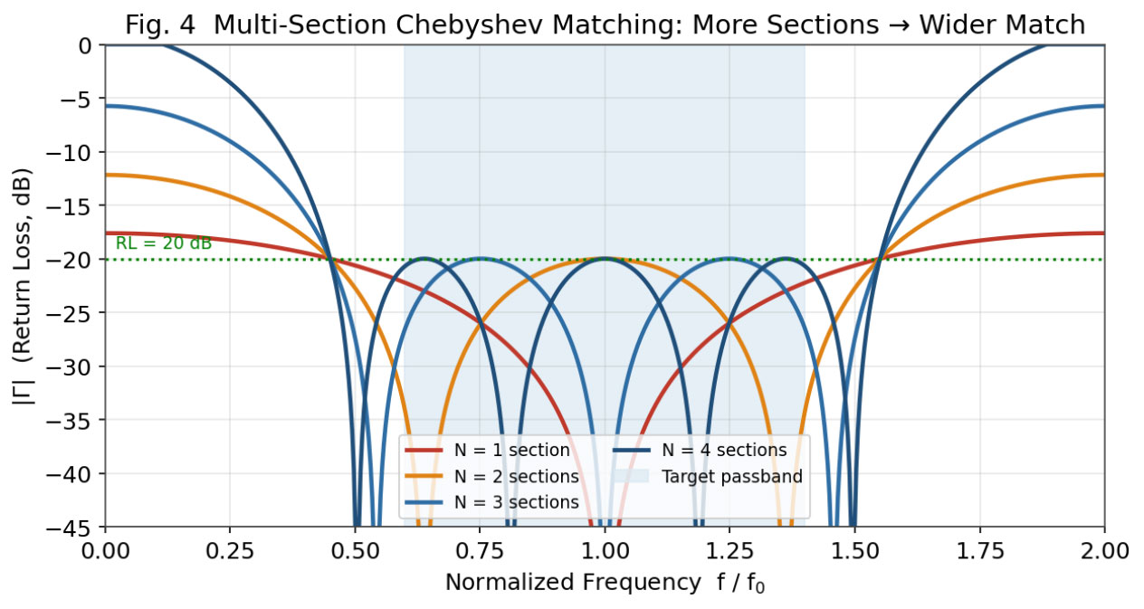
The Chebyshev multi-section transformer replaces a single section with N stepped transmission-line sections whose impedances follow a Chebyshev polynomial, giving an equiripple reflection response in band.^[8][9][10]

Wider matching bandwidth than a binomial transformer for the same N.
Precisely controllable in-band ripple, equivalent to a VSWR bound.
Bandwidth keeps extending with N, approaching the Bode–Fano limit.

A 3-section transformer (50 Ω → 100 Ω, Γ_m = 0.05) yields Z₁ = 57.37 Ω, Z₂ = 70.71 Ω, Z₃ = 87.15 Ω.^[10]

Fig. 4 Multi-section Chebyshev matching: more sections → wider match (equiripple, N = 1–4).

In wideband cavity filters this is realized via tapered coupling-aperture sizing, stepped coupling-probe lengths, and multi-section quarter-wave transformers between connector and cavity.^[7]

4.2 Tapered (Taper) Structures

For a more continuous, compact match, the tapered transmission line varies Z(z) smoothly from Z₀ to Z_L.^[11][12][10]

Table 2. Comparison of common taper types

Taper Type	Impedance Profile	Characteristics	Use Case
Exponential	Z(z)=Z₀·e^(az)	Simple; out-of-band ripple	General wideband use
Triangular	Linear ln Z profile	Good low-pass cutoff	Moderate-bandwidth use
Klopfenstein	Chebyshev-optimized	Shortest length for given Γ	High-demand UWB

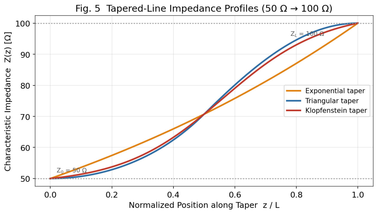
Fig. 5 Tapered-line impedance profiles (50 Ω → 100 Ω): Klopfenstein is shortest for a given reflection.

The Klopfenstein taper provides the shortest length for a specified in-band reflection, the optimal UWB choice. Recent work shows an exponential taper with shaping-factor optimization can be more compact than a linear taper while keeping VSWR < 1.1.^[11]

4.3 Integrated Design Flow

Recommended design flow

(1) Choose Chebyshev order N and ripple spec → (2) Design each cavity coupling iris/probe from the coefficients → (3) Apply a taper at the connector ends for final transition → (4) Optimize with HFSS/CST full-wave simulation → (5) Compare measured S-parameters and apply mechanical tuning.

5. Temwell UWB Products: Cavity BPF Specifications

5.1 Product-Line Overview

The Temwell UWB cavity bandpass filter series covers 500 MHz–28 GHz for telecom, satellite, radar, base-station, and aerospace applications.^[2]

Table 3. Main standard Temwell UWB cavity bandpass filter models

Model	Type	Center Freq.	Passband (MHz)	BW (MHz)	IL (dB)	VSWR
ST-WB01-500S	LC BPF	500 MHz	200–800	600	8.0	1.8:1
ST-WB03-1450S	LC BPF	1450 MHz	500–2400	1900	1.5	1.7:1
ST-WB05-3000S	Interdigital	3000 MHz	2125–3875	1750	1.0	1.5:1
ST-WB06-5000S	Interdigital	5000 MHz	3650–6350	2700	1.0	1.5:1
ST-WB07-7000S	Interdigital	7000 MHz	5650–8350	2700	1.0	1.5:1
ST-WB08-9000S	Interdigital	9000 MHz	8000–10000	2000	1.0	1.5:1
ST-WB15-26GK	Cavity BPF	26875 MHz	24250–29500	5250	1.0	RL≥14 dB
ST-WB16-28GK	Cavity BPF	28000 MHz	26500–29500	3000	1.0	RL≥15 dB

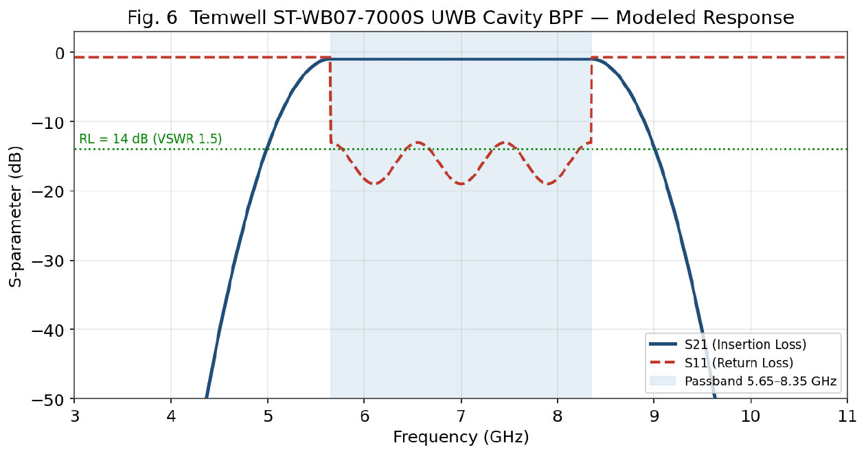
5.2 Representative Case: ST-WB07-7000S

Table 4. ST-WB07-7000S detailed specification

Parameter	Specification
Center frequency	7.0 GHz
Passband bandwidth	2700 MHz (5.65–8.35 GHz), FBW ≈ 38.6%
Insertion loss	≤ 1.0 dB
Passband VSWR	≤ 1.5:1 (RL ≥ 14 dB)
Stopband attenuation	≥ 40 dB @ f₀ ± 2500 MHz
System impedance / connector	50 Ω / SMA-Female
Operating temperature	−40°C to +70°C

Fig. 6 Temwell ST-WB07-7000S UWB cavity BPF — modeled S-parameter response (S21 / S11).

5.3 How Matching Design Affects Insertion Loss

Temwell documentation shows insertion loss is inversely related to bandwidth: BW < 10 MHz gives IL ~2.0–5.0 dB; BW > 100 MHz gives IL < 1.0 dB with smaller group delay (< 10–20 ns). This agrees with Bode–Fano — a wideband cavity filter maintains or improves IL while widening the band by using multi-cavity coupling instead of very high-Q resonance.^[15]

6. System Integration: Matching Verification with Amplifiers and Antennas

6.1 System-Level Principles

With amplifiers: PA output impedance varies with frequency and may deviate from 50 Ω; LNA input is complex and needs noise-optimum matching. By Bode–Fano, the gain-bandwidth product has a ceiling; over-demanding matching bandwidth sacrifices gain.^[3]

With antennas: an antenna is a reactive (high-Q) load; UWB antenna matching bandwidth is Bode–Fano-bounded. Ground plane and surrounding metal affect input impedance and require re-verification after integration.

6.2 Verification Methods

VNA S-parameters: after SOLT/TRL calibration, measure S11/S22 (RL ≥ 14 dB), S21, group delay, and export S2P.
TDR: locate local impedance discontinuities (connectors, joints) in the time domain.^[13]
Load Pull: map the PA optimum power-output impedance and confirm the filter input falls inside the constant-power circle.^[3]
Link-budget check: estimate system impact via mismatch loss (VSWR 1.5 → 0.18 dB; 2.0 → 0.51 dB, see Fig. 2).

6.3 Common Integration Problems and Solutions

Table 5. Common integration problems and fixes

Symptom	Possible Cause	Solution
VSWR degrades in part of band	Connector-interface discontinuity	Replace connector; improve soldering
Frequency-dependent IL ripple	Box-mode resonance	Add absorber or adjust enclosure
S11 drift over temperature	Thermal expansion alters coupling	Low-CTE materials / temp compensation
Gain ripple after PA connection	Amplifier reflection affects filter	Add isolator/circulator at interface
Band shift after antenna integration	Antenna–filter interaction	Re-optimize with full system model

7. Conclusion: Key Points for UWB Selection

Impedance-matching design for UWB cavity bandpass filters is an engineering optimization within the Bode–Fano physical limit. The core logic:

1. Accept the match–bandwidth trade-off

For UWB, VSWR ≤ 1.5:1 is the practical standard balancing bandwidth, loss, and complexity.

2. Prefer multi-section Chebyshev

An N ≥ 3 Chebyshev network gives the best bandwidth extension with controllable ripple.

3. Klopfenstein taper is optimal

For size-constrained cases it is the shortest design meeting a specified VSWR bound.

4. Full-wave simulation is mandatory

Cavity distributed effects are non-negligible at GHz; verify with HFSS/CST.

Temwell UWB Selection Guide

Table 6. Selection guide by application

Application Scenario	Recommended Series	Key Metrics
5G/6G Sub-6 GHz base station	ST-WB05 / ST-WB06	IL ≤ 1.0 dB, VSWR ≤ 1.5:1
5G mmWave 26–28 GHz	ST-WB15 / ST-WB16	IL ≤ 1.0 dB, RL ≥ 14–15 dB, K-type conn.
X-Band radar (9 GHz)	ST-WB08-9000S	IL ≤ 1.0 dB, stopband ≥ 60 dB
Satellite C-Band receive	ST-WB06-5000S	Wide 2700 MHz BW, low-noise
Wideband instrumentation	ST-WB02-515N	30–1000 MHz ultra-wide passband
Electronic warfare / SIGINT	Custom design	DC–60 GHz, multi-band coverage

This paper is based on public academic literature and official Temwell Corporation product data; all specifications are subject to the latest Temwell datasheets.

★ References

Back