

Impact of Mechanical Tolerance on Return Loss and Bandwidth in Waveguide Cavity Filters

A waveguide filter is asked to deliver low insertion loss, high power handling and sharp selectivity at the same time, yet whether it meets its electrical specification is ultimately decided by the dimensional accuracy of machining and assembly. This study takes a WR-28 (Ka-band) four-pole Chebyshev waveguide bandpass filter as its worked example (f0 = 30 GHz, BW = 800 MHz, design return loss 22 dB), separates the three classes of tolerance source — CNC machining accuracy, assembly error and surface roughness — and quantifies their electrical consequences with a coupling-matrix model. The analysis shows that for the same absolute tolerance the relative frequency shift scales inversely with the waveguide broad-wall dimension: a ±25 μm deviation produces only a 0.12% centre-frequency shift at X-band but 1.07% at W-band. For the Ka-band example here, ±25 μm corresponds to a 106 MHz downward shift — about 13% of the 800 MHz passband, equivalently 27% of the 400 MHz half-bandwidth. Sensitivity analysis identifies the inner resonators (cavities 2 and 3) as roughly 1.7 times more critical to return loss than the outer ones, while coupling-iris errors act mainly on bandwidth rather than S11: for a thin-wall narrow inductive iris of nominal opening w = 3.5 mm, a ±15 μm deviation corresponds to about ±1.3% coupling variation and ±1.6% deviation of the 3 dB bandwidth. Monte Carlo statistics (1,500 trials per case) show that without tuning, even holding critical cavity dimensions to ±10 μm (3σ) yields only about 14% of units at RL ≥ 20 dB; introducing per-cavity tuning-screw compensation restores the yield to 100% at the same tolerance, and still holds 95% at ±25 μm. The conclusion is that for millimetre-wave waveguide filters, machining tolerance and tunable design are not alternatives but two lines of defence that must be planned together. The paper further presents Temwell's dimensional tolerance specification, CMM and VNA outgoing acceptance flow, field frequency-tuning method, and the checklist of mechanical specifications and quality documents a buyer should request from a supplier.
1. Introduction
1.1 The role of waveguide filters in mmWave and microwave systems
The waveguide filter is one of the most critical passive components in millimetre-wave (mmWave) and microwave systems: it passes a designated band while suppressing out-of-band noise and interference. Compared with microstrip or coaxial structures, the rectangular metallic waveguide filter offers three advantages that are hard to replace. First, the interior is air-filled, so there is no dielectric loss and a very high unloaded quality factor (Q_u) can be maintained at high frequencies, giving extremely low insertion loss. Second, the large cross-section spreads the electric field, so power handling far exceeds that of planar circuits, making it suitable for radar transmitters and satellite amplifiers. Third, the passband skirts are steep and out-of-band rejection is excellent, giving high selectivity.
The common price of these three advantages is that the electrical performance of a waveguide filter is determined almost entirely by the geometry of its metal structure. Unlike a lumped circuit, where component values can be adjusted, the resonant frequency of each cavity, the inter-cavity coupling and the input/output external Q are all written into the length, width, depth and iris opening of the machined part. Mechanical tolerance in machining and assembly is therefore not a manufacturing quality issue downstream of design; it is a first-order design variable that decides whether the filter can meet its specification at all.
| Application | Typical band | Key performance requirement | Tolerance sensitivity |
|---|---|---|---|
| 5G / 6G mmWave base station | 24–100 GHz | Low loss, narrow band, high isolation | High |
| Satellite communication (SATCOM) | Ku / Ka band | Low return loss, temperature stability | High |
| Weather and military radar | X / Ku / W band | High power, tight frequency accuracy | Very high |
| Test and measurement | DC – 110 GHz+ | Reproducibility of frequency response | Very high |
Two metrics run through this paper. Return loss (RL) quantifies impedance match at the input: a higher value (say RL > 20 dB) means less reflected energy, higher power transfer efficiency, and protection of the upstream power amplifier from reflected signal. Bandwidth (BW) determines the usable spectrum of the channel and the out-of-band rejection available. This paper shows that the two metrics are governed by different classes of mechanical tolerance: return loss is driven mainly by cavity dimensional error (i.e. frequency error), while bandwidth is driven mainly by coupling-iris dimensional error. Recognising this division of labour is what allows a tolerance budget to be spent where it matters.
1.2 Objectives and worked example
The objectives of this study are: (1) to organise the three classes of mechanical tolerance source in a waveguide filter and their physical origins; (2) to quantify, with a coupling-matrix model, how dimensional deviation affects centre frequency, return loss and bandwidth, and to rank the sensitivity of each parameter; (3) to establish a standard Monte Carlo yield analysis flow that links a tolerance grade directly to a production yield; (4) to present Temwell's dimensional tolerance specification and outgoing test flow; (5) to describe the field frequency-tuning method and the limits of its validity; and (6) to summarise the mechanical specifications a buyer should require from a supplier.
2. Three Classes of Mechanical Tolerance Source
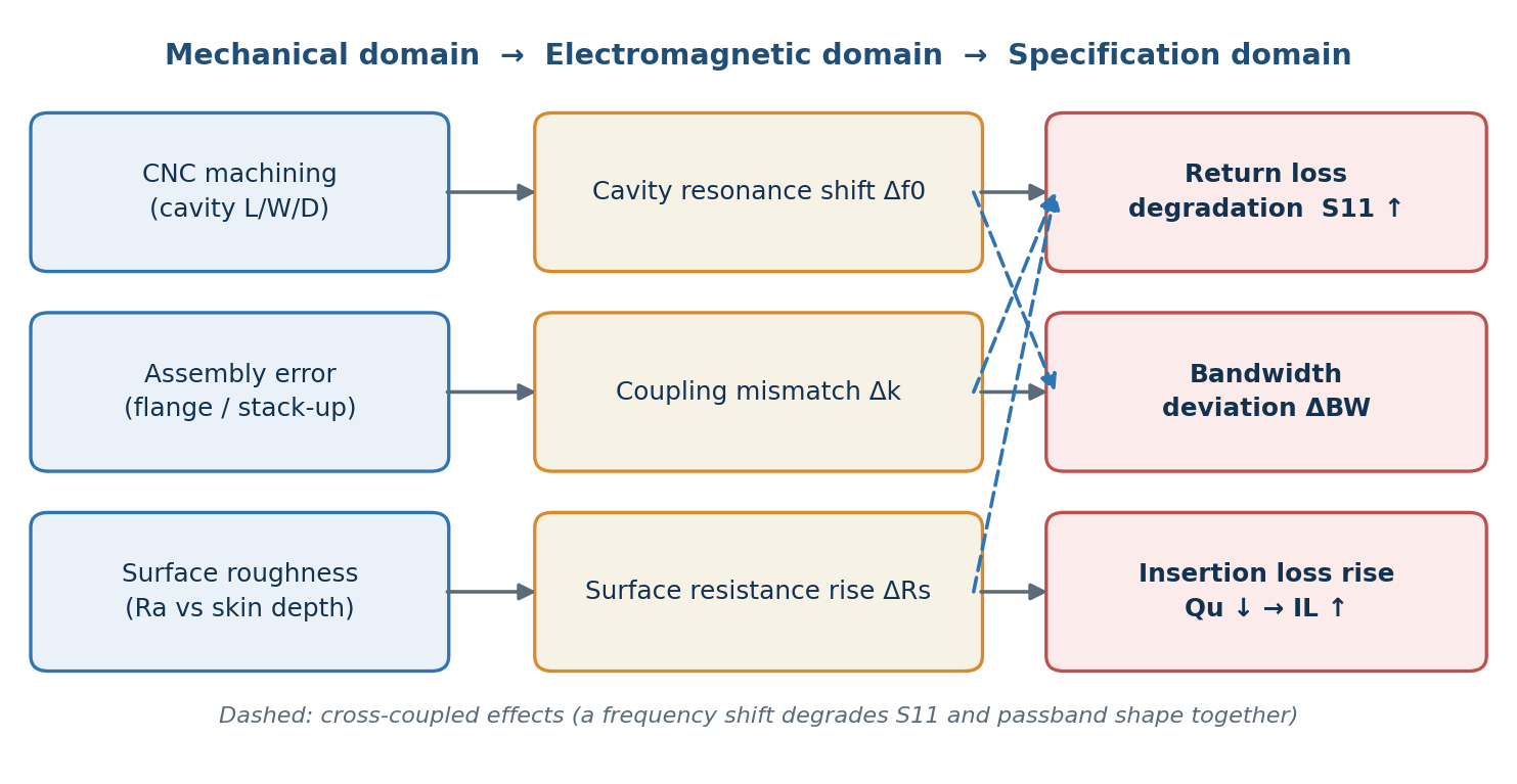
The mechanical tolerances of a waveguide filter fall into three classes, each acting on a different electrical parameter through a different physical path (Fig. 1). Separating this mechanical-domain to electromagnetic-domain to specification-domain chain is what allows an engineer to decide which process step to inspect when a particular specification is missed.
2.1 CNC machining accuracy
The cavities of a rectangular waveguide filter are usually milled from an aluminium alloy such as 6061-T6 or from OFHC copper, then silver- or gold-plated according to the frequency band. Machining accuracy depends jointly on machine rigidity, tool wear, thermal distortion from cutting and the repeatability of the fixture. Tool wear and thermal distortion are systematic in character — a whole batch drifts in the same direction — whereas fixture positioning error is closer to random. The two error types affect yield in very different ways, as Section 4 shows.
| Tolerance grade | Typical deviation | Applies to | Recommended band |
|---|---|---|---|
| General machining | ±0.10 – 0.25 mm | Outline, non-critical features | Any |
| Precision machining | ±0.025 – 0.05 mm | Cavity L/W/D, iris opening | < 20 GHz |
| High-precision machining | ±0.010 – 0.025 mm | Critical RF features | 20 – 60 GHz |
| Ultra-precision machining | ±0.005 – 0.010 mm | Coupling faces, cavity depth | > 60 GHz |
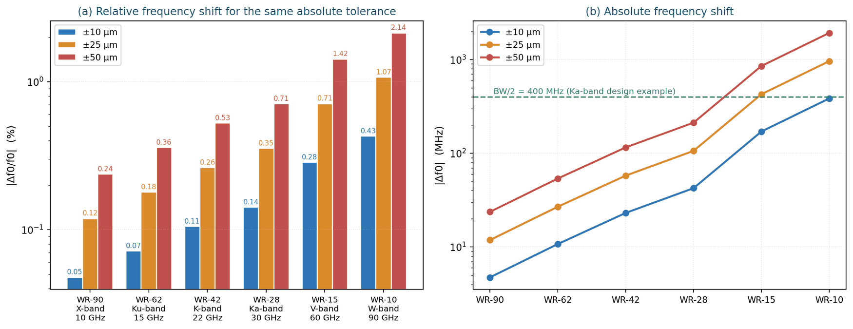
It is worth stressing that Table 2 is not a cost ladder in which tighter is always better; the thresholds are set by physics. Section 3 shows that the same absolute ±25 μm tolerance produces only a 0.12% frequency shift at X-band but 1.07% at W-band, simply because the waveguide shrinks with frequency and the relative error grows accordingly. This is the fundamental reason a millimetre-wave waveguide filter costs far more than a coaxial cavity filter of the same pole count.
2.2 Assembly error
A waveguide filter is normally assembled from several machined parts — cavity body, cover plate and flanges — and the assembly stage introduces its own errors:
- Flange misalignment — deviations in the parallelism and perpendicularity of the flange face create an electromagnetic discontinuity at the joint, which appears directly as additional reflection. At millimetre-wave frequencies a misalignment of tens of micrometres is enough to produce measurable S11 degradation.
- Tolerance stack-up — with several cavities in cascade, individual dimensional errors accumulate along the axis. If the errors share a direction (systematic error) the accumulation appears as an overall frequency shift; if their directions are random it appears as passband distortion and degraded in-band ripple.
- Uneven bolt torque — differences in bolt torque cause small elastic deformation of the flange face and change the effective cavity dimension. This error is especially common after a unit has been opened for service, and is a frequent cause of performance being worse after repair than at delivery.
- Joint stress and brazing distortion — with soldering or diffusion bonding, thermal stress can leave residual distortion in the cavity, and that distortion may continue to relax over subsequent temperature cycles.
2.3 Surface roughness
Surface roughness is the only one of the three tolerance classes that does not shift the resonant frequency, yet it erodes Q_u and conductor loss directly. The mechanism is the skin effect: RF current flows only within a very thin skin depth at the conductor surface,
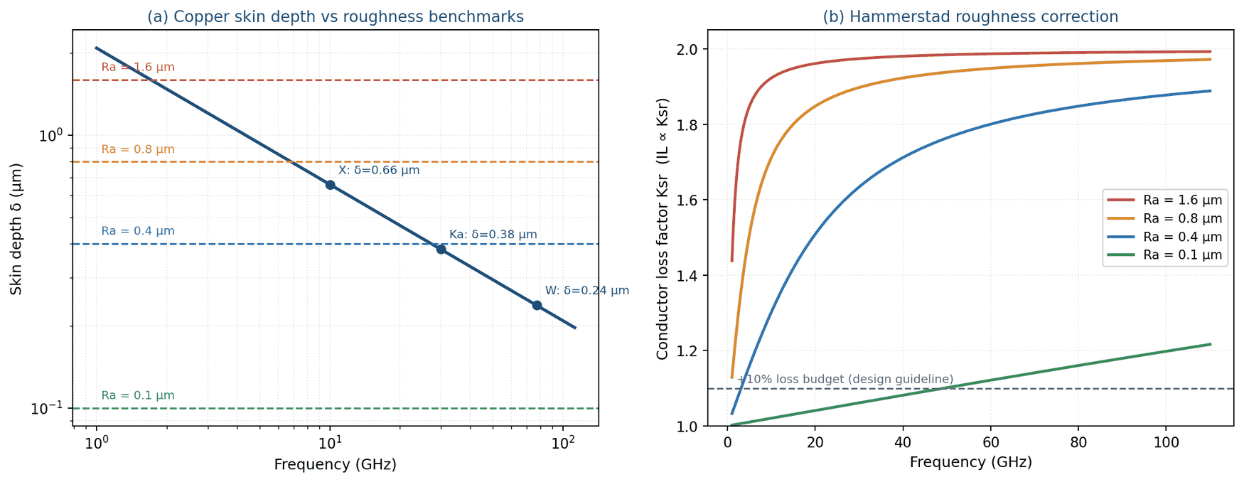
where δ is skin depth, ρ conductor resistivity, f operating frequency, μ0 the permeability of free space and μr the relative permeability. For copper (ρ = 1.72 × 10⁻⁸ Ω·m) the skin depth is about 0.66 μm at 10 GHz, 0.38 μm at 30 GHz and only about 0.24 μm at 77 GHz (Fig. 4a). Once the arithmetic mean roughness Ra approaches or exceeds δ, the current is forced to follow the rough profile, its effective path lengthens and the effective surface resistance rises. In engineering practice this is described by the Hammerstad correction factor:
It should be stressed that K_sr scales the conductor surface resistance and conductor loss, not the total insertion loss directly; how much the total IL rises depends on the fraction of total loss attributable to conductor loss (in an air-filled waveguide conductor loss dominates, so the two are close, but they are not identical). On this model (copper, 30 GHz, Hammerstad), a surface with Ra = 0.8 μm multiplies conductor loss by about 1.90 and Ra = 0.4 μm by 1.63; keeping the roughness-induced increase in conductor loss within 10% requires Ra of order 0.13 μm or below (Fig. 4b). In other words, the internal surface condition of a millimetre-wave waveguide filter matters no less than the cavity dimensions themselves — which is why high-frequency waveguide components are often produced by electroforming, or by fine polishing followed by plating.
| Surface finish | Ra | Ra/δ at 30 GHz | Conductor loss factor K_sr | Suitable band |
|---|---|---|---|---|
| Standard CNC milling | 3.2 μm | 8.4 | ≈ 2.0 | < 6 GHz |
| Precision milling | 1.6 μm | 4.2 | 1.97 | < 12 GHz |
| Precision machining + plating | 0.8 μm | 2.10 | 1.90 | 12 – 30 GHz |
| Ultra-precision polish + silver plating | 0.4 μm | 1.05 | 1.63 | 30 – 60 GHz |
| Electroforming / optical-grade polish | < 0.1 μm | 0.26 | 1.06 | > 60 GHz |
3. Electrical Consequences of Mechanical Tolerance
3.1 Quantifying the frequency shift
The TE101 resonant frequency of a rectangular waveguide cavity is set by the broad-wall dimension a and the cavity length d:
This expression assumes an idealised air-filled rectangular cavity in the TE101 mode with the height b neglected, and serves as a first-order geometric sensitivity model; a realised filter is additionally affected by iris loading, tuning elements, plating and assembly interfaces, so its absolute resonant frequency must be calibrated by full-wave simulation or measurement. The sensitivity trend derived below — relative frequency shift scaling inversely with the broad-wall dimension — nonetheless survives those corrections. Taking the total differential gives the first-order relation between dimensional deviation and frequency shift. If all dimensions shift by the same absolute amount Δ — the usual case for one tool and one fixture — then
The sensitivity coefficient S has dimensions of inverse length and is numerically close to 1/a. This expresses one key fact: the same absolute machining tolerance produces a larger relative frequency shift the higher the band, because the broad wall a shrinks in inverse proportion to frequency. For the WR-28 example here, a = 7.112 mm and d = 7.021 mm give S = 0.1415 mm⁻¹, so every 10 μm of dimensional deviation corresponds to a 0.142% centre-frequency shift — 42 MHz at 30 GHz. Table 4 and Fig. 2 give the full comparison across six standard waveguide bands.
| Waveguide | Band | f0 | a (mm) | S (mm⁻¹) | Δf0 @ ±10 μm | Δf0 @ ±25 μm | Δf0 @ ±50 μm |
|---|---|---|---|---|---|---|---|
| WR-90 | X | 10 GHz | 22.860 | 0.0475 | 0.048% / 5 MHz | 0.119% / 12 MHz | 0.238% / 24 MHz |
| WR-62 | Ku | 15 GHz | 15.799 | 0.0718 | 0.072% / 11 MHz | 0.180% / 27 MHz | 0.359% / 54 MHz |
| WR-42 | K | 22 GHz | 10.668 | 0.1051 | 0.105% / 23 MHz | 0.263% / 58 MHz | 0.526% / 116 MHz |
| WR-28 | Ka | 30 GHz | 7.112 | 0.1415 | 0.142% / 42 MHz | 0.354% / 106 MHz | 0.708% / 212 MHz |
| WR-15 | V | 60 GHz | 3.759 | 0.2845 | 0.284% / 171 MHz | 0.711% / 427 MHz | 1.422% / 853 MHz |
| WR-10 | W | 90 GHz | 2.540 | 0.4277 | 0.428% / 385 MHz | 1.069% / 962 MHz | 2.138% / 1925 MHz |
Two error types must be distinguished here, because their consequences and their remedies are entirely different:
- Systematic (correlated) error — all cavities shift in the same direction. The response shape is preserved and only the centre frequency translates. This class can be corrected by global tuning or design compensation; in yield terms it appears as a frequency-out-of-spec failure rather than a shape failure.
- Random (uncorrelated) error — each cavity deviates independently. The spread of resonant frequencies distorts the passband shape, worsens in-band ripple and flattens out the group delay, and cannot be corrected by a single global adjustment; each cavity must be compensated individually.
3.2 The mechanism of return loss (S11) degradation
Return loss does not degrade as a direct consequence of dimensional error but through a clear causal chain: dimensional deviation shifts the cavity resonance, the coupling coefficients become mismatched relative to their design values, an impedance discontinuity appears at the passband edge, and reflected power increases. Simulating the Ka-band example with the coupling-matrix model and reading the worst return loss inside the fixed specification band (30.0 ± 0.4 GHz) gives Table 5.
| Uniform deviation | Centre-frequency shift | Worst in-band RL | Verdict (RL ≥ 20 dB) |
|---|---|---|---|
| 0 μm (ideal) | 0 MHz | 21.1 dB | Pass |
| ±5 μm | 21 MHz (0.071%) | 16.8 dB | Fail |
| ±10 μm | 42 MHz (0.141%) | 12.6 dB | Fail |
| ±15 μm | 64 MHz (0.212%) | 9.5 dB | Fail |
| ±25 μm | 106 MHz (0.354%) | 5.1 dB | Severe fail |
| ±50 μm | 212 MHz (0.708%) | 0.9 dB | Passband out of band |
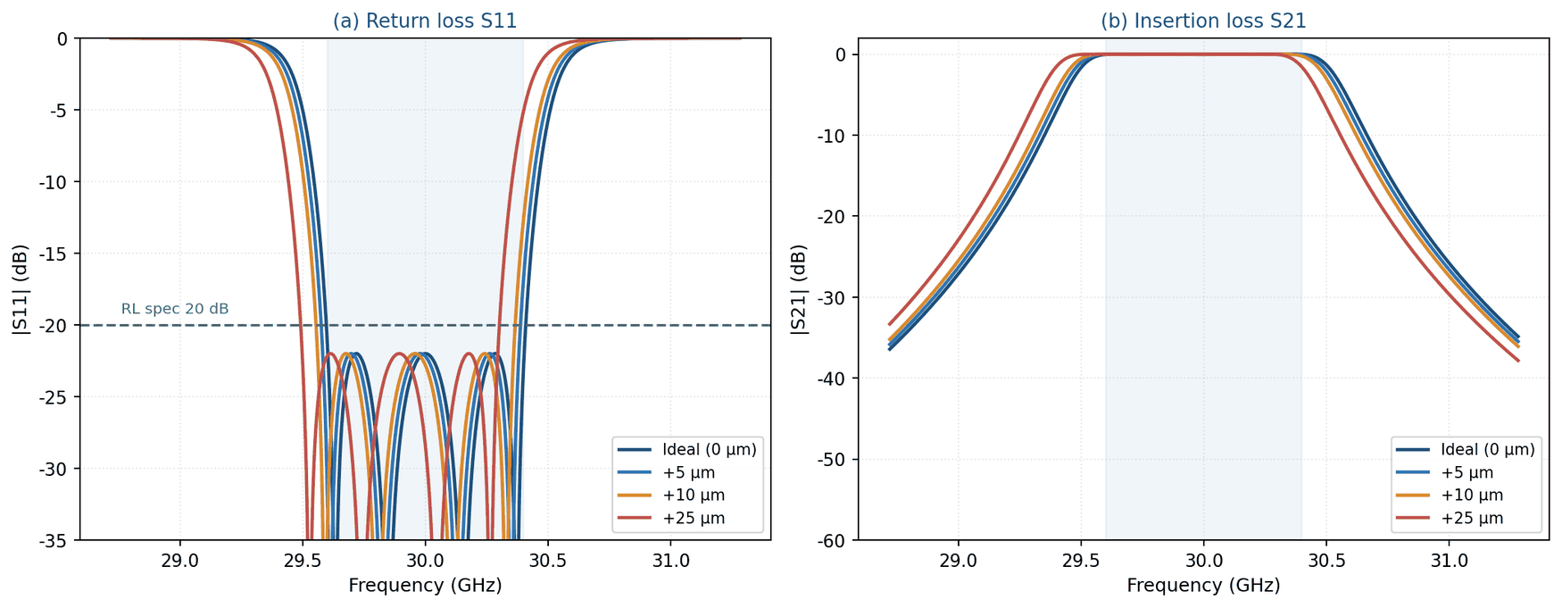
The figures in Table 5 look severe and must be read correctly: they measure the as-machined result with no tuning at all, against a fixed specification window. If the centre frequency is allowed to be redefined globally — that is, if the system can accept a frequency translation — the response shape of the same parts is in fact intact. This is the concrete expression of the rule that systematic error is compensable and random error is not. What actually determines yield is the sensitivity distribution of Section 3.3 and the random statistics of Section 4.
3.3 Sensitivity ranking: where the tolerance budget should go
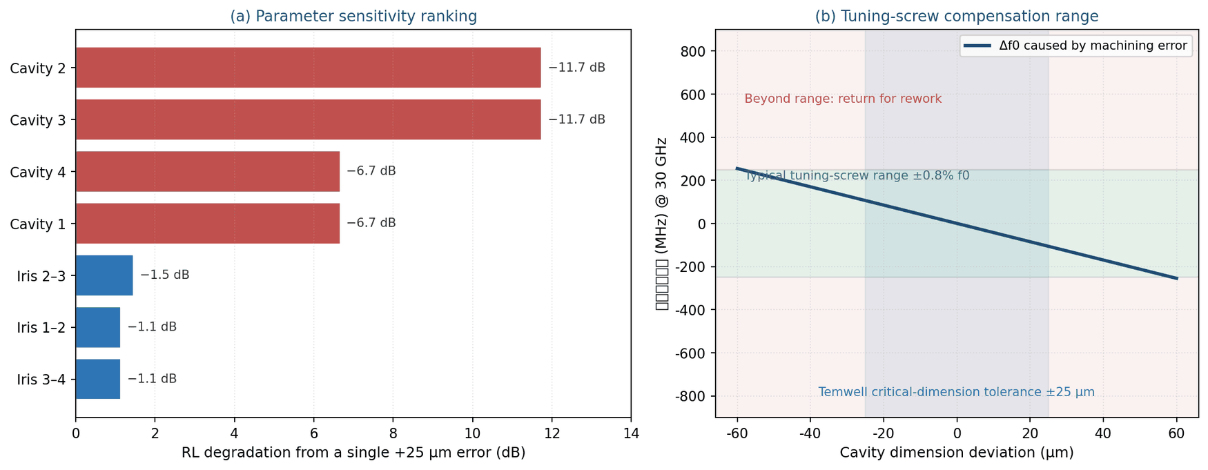
Not all dimensions matter equally. Scanning the four-pole example with a single-parameter perturbation — deviating one dimension by +25 μm at a time while the others stay nominal — gives the sensitivity ranking in Fig. 6a and Table 6. Two clear patterns emerge:
- Cavity dimensional error dominates return loss — for the four-pole Chebyshev example of this paper, a single +25 μm deviation on an inner cavity (2 or 3) degrades return loss from 21.1 dB to 9.4 dB (an 11.7 dB drop), while the same deviation on an outer cavity (1 or 4) degrades it to 14.4 dB (a 6.7 dB drop) — the inner cavities are about 1.7 times more sensitive. Qualitatively this is because each inner cavity participates in two coupling nodes, so its detuning breaks the match on both sides at once. The ratio of 1.7 itself, however, depends on the coupling-matrix topology, pole count, coupling distribution, external Q and response type (Chebyshev, quasi-elliptic, cross-coupled), and is not a universal property of waveguide filters; it must be recomputed for each design.
- Iris dimensional error dominates bandwidth, not S11 — the same +25 μm deviation on an iris opening degrades return loss by only 1.1–1.5 dB, but it changes the coupling coefficient and hence the passband width. For a thin-wall, narrow, weakly coupled inductive iris the aperture-polarisability approximation gives a leading-order dependence k ∝ w³ (w being the iris opening width), so that for small perturbations Δk/k ≈ 3·(Δw/w). Taking the nominal opening used here, w = 3.5 mm, a ±15 μm iris deviation corresponds to about ±1.3% coupling variation and about ±1.6% deviation of the 3 dB bandwidth; ±30 μm corresponds to roughly ±3.2%. Note that k ∝ w³ is not a universal design law for waveguide irises — actual coupling also depends on iris thickness, wall thickness, aperture shape, cavity height and whether the iris is capacitive or inductive — so the real sensitivity should be extracted from EM simulation or prototype tuning before production.
| Parameter | Worst RL at +25 μm | Degradation | Primary metric affected |
|---|---|---|---|
| Cavity 2 / Cavity 3 (inner) | 9.4 dB | −11.7 dB | Return loss |
| Cavity 1 / Cavity 4 (outer) | 14.4 dB | −6.7 dB | Return loss |
| Iris 2–3 (centre) | 19.6 dB | −1.5 dB | Bandwidth |
| Iris 1–2 / 3–4 | 20.0 dB | −1.1 dB | Bandwidth |
This ranking has a direct cost implication: rather than applying ultra-precision tolerance uniformly to every dimension, machining resource should be concentrated on the critical dimensions of the inner cavities, while iris openings can carry a looser tolerance backed by subsequent tuning. This is the most useful engineering output of a Monte Carlo analysis — not a yield number, but a tolerance budget allocation.
4. Tolerance Analysis: Monte Carlo Statistical Yield Study
4.1 Methodology
Monte Carlo analysis is the standard statistical tool for assessing how manufacturing tolerance affects the electrical performance of a waveguide filter. Random perturbations are applied simultaneously to every tolerance-affected geometric parameter, the simulation is repeated some thousands of times, and the manufacturing yield is estimated from the statistical distribution of the results. Its advantage over single-parameter worst-case analysis is that worst-case assumes every error takes its extreme value in the least favourable direction at once — statistically a very rare event — which drives tolerance requirements to be over-conservative and raises cost for no return.
4.2 Standard workflow
- Define the tolerance variables and their probability distributions — list every critical dimension (cavity length, width and depth, iris opening, wall thickness, flange flatness) and assign a distribution to each. Use actual measurement data from statistical process control (SPC), not an arbitrary uniform assumption.
- Build the EM or circuit model — a full-wave model in HFSS/CST, or a reduced-order coupling-matrix model. Full-wave models are accurate but slow per iteration; in practice a small number of full-wave runs is used to calibrate a coupling matrix, and the bulk of the trials is then run on the matrix.
- Run the random trials — about 1,000 trials suffice for an engineering estimate; 10,000 or more is recommended before a final design decision, so that the yield estimate has converged.
- Compute the yield — classify each trial against pre-defined pass/fail criteria, Yield = N_pass / N_total × 100%. The criteria should combine insertion loss, return loss, bandwidth and out-of-band rejection rather than any single metric.
- Sensitivity analysis and tolerance reallocation— identify the dominant tolerance drivers, tighten those dimensions specifically, and relax the non-critical ones, to reach the best balance of yield against cost.
4.3 Yield results for the worked example
Monte Carlo analysis of the four-pole Ka-band example: cavity dimensional errors are normally distributed, N(0, σ²) with σ = T/3 for a nominal tolerance T, independent per cavity; the standard deviation of the iris error is set to 0.6 times that of the cavity error. Each tolerance grade is run for 1,500 trials, with the criterion taken as the worst return loss inside the specification band (30.0 ± 0.4 GHz). Three scenarios are compared: no tuning, global frequency retune only, and per-cavity tuning-screw compensation. Results are given in Table 7 and Fig. 5.
| Cavity tolerance (3σ) | As-machined RL ≥ 20 dB | As-machined RL ≥ 15 dB | Global retune RL ≥ 20 dB | Per-cavity tuning RL ≥ 20 dB |
|---|---|---|---|---|
| ±5 μm | 50.4 % | 100 % | 77.5 % | 100 % |
| ±10 μm | 13.9 % | 93.5 % | 30.8 % | 100 % |
| ±15 μm | 4.2 % | 76.1 % | 12.7 % | 99.6 % |
| ±25 μm | 0.7 % | 34.9 % | 2.7 % | 95.3 % |
| ±50 μm | 0.1 % | 5.4 % | 0.4 % | 67.4 % |
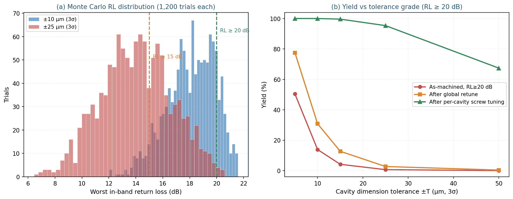
Three points summarise Table 7. First, above Ka-band, machining accuracy alone cannot deliver a production yield at 20 dB return loss: even tightening the tolerance to ±5 μm, which is already ultra-precision territory, leaves the untuned yield at 50%. Second, a global frequency retune helps only modestly, because it corrects systematic error alone and can do nothing about the passband distortion produced by independent cavity-to-cavity scatter — at ±10 μm it lifts the yield only from 13.9% to 30.8%. Third, per-cavity tuning-screw compensation is the decisive measure: it allows each resonant frequency to be corrected independently and holds the yield at 95.3% even with a ±25 μm tolerance. This is why many commercial waveguide bandpass filters with tight frequency and match specifications incorporate tuning structures — for such specifications tunability is less an option than a precondition for yield. (Fixed, once-calibrated, monolithic or additively manufactured designs do not necessarily use tuning screws.)
5. Temwell Manufacturing Control: Dimensional Specification and Outgoing Test Flow
5.1 Machining tolerance specification
Temwell's Standard Waveguide Filter series allocates its tolerance budget according to the sensitivity ranking of Section 3: the tightest tolerance goes to the cavity dimensions that dominate return loss, the iris openings come next, and non-RF outline dimensions carry general machining tolerance — balancing yield against cost.
| Feature class | Tolerance | Measurement method | Control |
|---|---|---|---|
| Cavity critical dimensions (L/W/D) | ±0.010 – 0.025 mm | CMM | 100% or first article + sampling |
| Coupling iris opening | ±0.015 mm | Optical image measurement | 100% or first article + sampling |
| Flange flatness | ≤ 0.010 mm | Flatness gauge | 100% |
| Flange bolt circle (PCD) | ±0.025 mm | CMM | Sampling |
| Internal surface roughness (Ka-band) | Ra ≤ 0.8 μm | Surface roughness tester | Sampling |
| Outline dimensions | ±0.10 mm | Calliper / gauge | Sampling |
Complete measurement records are retained for every critical dimension, with batch traceability under an ISO 9001:2015 quality management system. The measurement data also feed back into the SPC database and become the distribution input for the next round of Monte Carlo analysis — so that tolerance setting is no longer an engineer's guess but a decision derived from demonstrated process capability.
5.2 Outgoing test flow
- VNA calibration — full two-port calibration by SOLT or TRL, with the reference plane set at the waveguide flange face. Millimetre-wave measurement requires waveguide calibration standards; the discontinuity of a coaxial adapter otherwise folds directly into the S11 reading.
- Full-band S-parameter sweep — measure S11 (verifying that in-band return loss is better than specification), S21 (verifying that in-band insertion loss is below specification), and confirm that out-of-band rejection meets the cut-off specification at the designated frequencies.
- Frequency response verification— confirm that the centre frequency lies within the permitted deviation of the design frequency and that the 3 dB bandwidth is within ±5% of specification.
- Tuning and locking — after the per-cavity tuning procedure of Section 6, tighten the tuning-screw lock nuts, apply thread-locking compound, and re-measure the S-parameters to confirm that the response has not drifted back.
- Environmental reliability sampling — temperature-cycle a proportion of each batch and re-measure the S-parameters afterwards, verifying the dimensional stability of the mechanical structure under thermal stress.
Test data are archived electronically, and a complete outgoing test report can be supplied with the product for incoming inspection at the customer. For high-reliability applications Temwell can additionally provide batch-to-batch S-parameter consistency statistics and a summary of the CMM measurement data.
6. Service Tuning: Field Frequency Adjustment
6.1 The physics of the tuning screw
When a waveguide filter drifts in frequency — through residual machining error, long service, transport vibration or ambient temperature change — a tuning screw allows fine adjustment without remachining the cavity. The screw enters through the centre of the broad wall and its effect depends on insertion depth:
- Shallow insertion (depth < λ/4) — the screw sits where the cavity electric field is strongest and acts as a capacitive load, shifting that cavity's resonance downward. This is the usual working range because it is the most linear and controllable.
- Deep insertion (approaching λ/4) — the inductive effect grows and the frequency starts to shift upward. This region is highly sensitive and non-monotonic and should be avoided in practice.
- Coupling screws — placed near the iris between adjacent cavities to trim the coupling coefficient and hence the bandwidth and in-band ripple. Used together with the cavity tuning screws they correct frequency and match simultaneously, much like a double-stub tuner.
6.2 Field tuning procedure
- Preparation — connect the VNA to both ports, perform a waveguide calibration with the reference plane at the filter flange, record the baseline S11 and S21, and photograph or note the initial position and lock state of every tuning screw.
- Locate each cavity resonance — with the other port suitably decoupled, measure the resonant frequency of each cavity in turn starting from the input, building a complete picture of which cavity has shifted and by how much before deciding the adjustment order.
- Tune cavity by cavity — work from input to output, bringing each resonance onto its target frequency. Each depth change should be less than 0.25 mm, with the VNA response watched in real time to avoid overshoot.: VSWR ≤ 1.5:1 (RL ≥ 14 dB).
- Trim the coupling — once all cavity frequencies are in place, adjust the inter-cavity coupling screws to optimise passband shape, in-band ripple and 3 dB bandwidth.
- Final verification and locking — confirm that centre frequency, in-band return loss, insertion loss and out-of-band rejection all meet specification, then tighten the lock nuts, apply thread-locking compound, and re-measure once more to confirm that locking has not shifted the response.
6.3 The limits of tuning
- The tuning range is finite — a tuning screw typically covers about ±0.5–1.0% of f0. For the Ka-band example here (taking ±0.8%) that is roughly ±240 MHz, corresponding to a recoverable machining error of about ±57 μm (Fig. 6b). Beyond that range, forcing the screw deeper severely degrades Q_u and power handling, and the cavity should be returned for remachining.
- Tuning costs Q — the screw itself introduces additional conductor loss and field perturbation, and the deeper it goes the more Q_u falls. Trading loose tolerance for heavy tuning is therefore not a free lunch; it shows up as increased insertion loss.
- Sensitivity is extreme at high frequency — above 40 GHz, an eighth of a turn can move the frequency by tens of megahertz. A micrometer tuner with live VNA monitoring is recommended.
- Locking is mandatory — always fit a lock nut or apply thread-locking compound after tuning. In a vibrating environment an unlocked screw gradually backs out, and this is one of the common causes of a unit that passed at the factory failing after installation.
7. Conclusions and Procurement Guidance
7.1 Conclusions
- The electrical consequence of tolerance is amplified with frequency — the relative frequency shift from a given absolute tolerance scales inversely with the waveguide broad wall. A ±25 μm deviation gives 0.12% at X-band but 1.07% at W-band. Millimetre-wave tolerance specifications cannot be carried over from microwave experience.
- Return loss and bandwidth are governed by different tolerances — cavity dimensional error dominates return loss (+25 μm degrades RL by 6.7–11.7 dB), while iris error dominates bandwidth (±15 μm corresponds to about ±1.6% of the 3 dB bandwidth) and moves RL by only 1–1.5 dB. The tolerance budget should be allocated accordingly rather than tightened uniformly.
- The inner cavities are the critical path — in a four-pole filter, cavities 2 and 3 are about 1.7 times more sensitive to return loss than cavities 1 and 4, because each participates in two coupling nodes. Machining resource should be concentrated there first.
- Machining accuracy alone cannot deliver millimetre-wave production yield — even at ±5 μm the untuned yield at RL ≥ 20 dB is only about 50%, whereas per-cavity tuning-screw compensation holds 95.3% at ±25 μm. Tunability is a precondition for yield, not an optional feature.
- Systematic and random error need separate management — systematic error (tool wear, thermal distortion) can be absorbed by a global retune or a design offset; random error (fixture positioning, assembly stack-up) can only be handled by per-cavity tuning or a tighter tolerance. A Monte Carlo analysis that ignores the correlation between them systematically overestimates yield.
- Surface roughness is an independent third path — it does not shift frequency but erodes Q_u and conductor loss directly through the skin effect. On the Hammerstad model (copper, 30 GHz), Ra = 0.8 μm multiplies conductor loss by about 1.9, and holding that increase within 10% requires Ra of order 0.13 μm or below. A specification that lists dimensional tolerance but omits surface roughness leaves an uncontrolled loss mechanism in place.
7.2 Waveguide filter procurement checklist
| Category | Item to verify | Recommended requirement | Why it matters |
|---|---|---|---|
| Electrical | Centre-frequency accuracy | Within ±0.1% | Directly reflects cavity dimensional control |
| Electrical | In-band return loss | RL ≥ 20 dB (application dependent) | Indicates cavity consistency and tuning quality |
| Electrical | 3 dB bandwidth tolerance | Within ±5% | Indicates iris machining accuracy |
| Mechanical | Cavity critical-dimension tolerance | ±0.025 mm (> 10 GHz) | The dominant driver of return loss |
| Mechanical | Coupling iris tolerance | ±0.015 mm | The dominant driver of bandwidth |
| Mechanical | Flange flatness and interface standard | ≤ 0.010 mm; specify WR plus UBR/CPR type | Joint discontinuity folds straight into S11 |
| Mechanical | Internal surface roughness | By band (Ka: Ra ≤ 0.8 μm) | Determines Q_u and insertion loss |
| Quality | CMM / optical measurement report | 100% first article plus batch sampling | The only objective evidence of a tolerance claim |
| Quality | VNA outgoing test report | Including full S-parameter traces | Directly comparable at incoming inspection |
| Quality | Monte Carlo yield analysis report | Recommended for high-reliability applications | Shows whether the supplier understands its own process capability |
| Maintenance | Tuning-screw specification and range | State the range as ±% of f0 | Sets the limit of what can be recovered in the field |
7.3 Temwell capabilities available today
| Capability | Technology / process | Customer value |
|---|---|---|
| Precision cavity machining | CNC milling with full CMM verification, ±0.010–0.025 mm on critical dimensions | Batch-to-batch frequency consistency |
| Tolerance and yield analysis | Coupling matrix plus Monte Carlo, driven by measured SPC distributions | Yield predicted before production, avoiding design iterations |
| Tunable structure design | Cavity and coupling tuning screws with a band-specific adjustment range | High yield maintained under a relaxed tolerance |
| Surface treatment | Precision machining plus silver or gold plating, Ra specified by band | Low insertion loss and long-term oxidation resistance |
| Full-band measurement | VNA waveguide calibration (SOLT/TRL) plus temperature-cycle sampling | A traceable outgoing test report |
| Custom filter design | Custom cavity topology from the customer's band, bandwidth, RL and space constraints | A single point of contact from design to production |
7.4 Twelve-month R&D roadmap
- Build an automated Monte Carlo flow driven by measured SPC distributions, replacing experience-based tolerance specifications with values derived from demonstrated process capability.
- Introduce a Ka-band (WR-28) standard waveguide bandpass filter line, and establish the 30 GHz measurement and tuning SOP that goes with it.
- Evaluate electroforming for V- and W-band products, targeting an internal surface roughness below Ra 0.1 μm.
- Extend automated tuning equipment to the waveguide product line, shortening per-cavity tuning time and improving batch consistency.
- Establish a standard batch-to-batch S-parameter consistency report as a standard deliverable for high-reliability customers in satellite and radar.
Appendix A Full Definition of the Model, Random Variables and Pass/Fail Criteria
This appendix collects the models, parameters and criteria behind every quantitative result in this paper so that a reader can check or reproduce them. All results are first-order design analysis, not measured data from finished units.
A.1 Filter synthesis and S-parameter model
- Topology — four-pole (N = 4) in-line coupled-resonator, no cross-coupling.
- Response — Chebyshev with 22 dB design return loss, corresponding to a passband ripple L_ar = 0.0275 dB. The lowpass prototype g-values are g0 = 1.000, g1 = 0.8539, g2 = 1.2707, g3 = 1.4900, g4 = 0.7283, g5 = 1.1726.
- Normalised coupling coefficients — M12 = M34 = 0.960, M23 = 0.727; external Q values qe1 = qe4 = 0.854 (normalised; the actual Qe = qe / FBW).
- Solution — Hong's coupling-matrix form, A = q + jλ·U − j·m, with λ = (1/FBW)·(f/f0 − f0/f), q = diag(1/qe1, 0, …, 0, 1/qeN), U the identity and m the coupling matrix including diagonal detuning terms; S21 = 2·[A⁻¹]_N1 / √(qe1·qeN) and S11 = 1 − 2·[A⁻¹]_11 / qe1. The numerically verified unitarity error is below 1×10⁻¹⁵.
- Model exclusions — this is a lossless (Q_u → ∞) first-order model and excludes conductor loss, iris loading, tuning screws and post perturbations, flange and cover seam parasitics, plating thickness and machining fillets. The passband S21 in Fig. 3(b) is therefore 0 dB; it shows passband shape and displacement only, and is not a prediction of actual insertion loss.
A.2 Mapping from dimensional deviation to electrical parameters
- Geometry — WR-28 with a = 7.112 mm and b = 3.556 mm; the cavity length d = 7.021 mm is back-calculated from the TE101 expression at f0 = 30 GHz. The nominal coupling-iris opening is w = 3.5 mm.
- Cavity dimension to resonant frequency — Δf0/f0 = −S·Δ with S = (a⁻³ + d⁻³)/(a⁻² + d⁻²) = 0.1415 mm⁻¹, assuming a and d shift by the same absolute amount Δ.
- Resonant frequency to coupling matrix — the normalised detuning of resonator i is written into the diagonal, m_ii = (2/FBW)·(Δf0i/f0).
- Iris opening to coupling coefficient — using the thin-wall narrow-slot weak-coupling aperture-polarisability approximation, k ∝ w³, so m_(i,i+1) = M0_(i,i+1)·(1 + 3·Δw/w).
A.3 Monte Carlo random variable settings
| Item | Setting |
|---|---|
| Cavity dimensional error distribution | Normal N(0, σ²) with σ = T/3, i.e. the nominal tolerance T corresponds to 3σ |
| Iris opening error distribution | Normal, with a standard deviation 0.6 times that of the cavity error |
| Correlation between variables | Errors of each cavity and each iris are assumed mutually independent (no correlation modelled) |
| Number of trials | 1,500 per tolerance grade (Table 7); the histograms in Fig. 5(a) use 1,200 per group |
| Random seed | Fixed seed, results reproducible |
| Frequency resolution | 5 MHz step over f0 × (1 ± 0.008) ± BW/2 |
A.4 Pass/fail criteria
- Specification window — 30.0 ± 0.4 GHz (that is, f0 ± BW/2), fixed and not moved with the unit under test.
- Primary criterion — the worst return loss inside the specification window must be ≥ 20 dB to pass; Table 7 also reports a relaxed ≥ 15 dB criterion for comparison.
- Criteria not included — insertion loss, out-of-band rejection and group delay are not checked simultaneously here. A production criterion should combine several metrics, so the yield figures in this paper should be read as an upper bound obtained with return loss alone.
A.5 Tuning models
- As-machined — the worst return loss is read directly from the machined result inside the fixed specification window.
- Global retune — the whole band is allowed to translate within f0 × (1 ± 0.008) and the best achievable worst-case return loss is taken. This models a compensation capability that can correct only a systematic frequency offset.
- Per-cavity tuning — the tuning screws are assumed able to restore every cavity resonance exactly to its design value (m_ii = 0), so that only the iris coupling deviation remains. This is an idealised upper bound: it excludes the Q_u reduction caused by screw insertion and the finite adjustment range.
- Tuning range — Fig. 6(b) uses ±0.8% of f0 as an estimate of a typical tuning-screw compensation range (±240 MHz at 30 GHz). The actual range depends on screw diameter and position, cavity geometry and the acceptable Q_u degradation, and must be confirmed case by case.
A.6 Surface roughness model
- Skin depth from δ = √(ρ/(π·f·μ0·μr)), with copper taken as ρ = 1.72 × 10⁻⁸ Ω·m and μr = 1.
- The roughness correction uses the Hammerstad empirical expression K_sr = 1 + (2/π)·arctan[1.4·(Ra/δ)²], applied to conductor surface resistance and conductor loss. It saturates at K_sr = 2 for large Ra/δ and is therefore a conservative upper bound; the Huray snowball model predicts a milder penalty for rough surfaces at high frequency.
- K_sr is a multiplier on conductor loss; the resulting increase in total insertion loss additionally depends on the fraction of total loss attributable to conductor loss.
A.7 Statement of applicable scope
The purpose of the models described in this appendix is to establish, at the design stage, a quantitative link from tolerance grade to electrical performance to yield, in support of tolerance budget allocation and specification negotiation. Their absolute values should not be quoted directly as product specifications. Any design entering production should have its model parameters calibrated by full-wave EM simulation, and its sensitivity and yield estimates verified on measured samples.
Appendix - Complete source FAQ
FAQ — Impact of Mechanical Tolerance on Return Loss and Bandwidth in Waveguide Cavity Filters (A-09)
This FAQ is compiled from the coupling-matrix model, Tables 1–10 and A1 and Figures 1–6 of this paper (Article No. A-09); the full model definition, random variable settings and pass/fail criteria are given in Appendix A. Unless otherwise noted, the values quoted are design-stage analysis and Temwell production experience, not the measurement report of any single unit. Actual product specifications are governed by the shipping test report.
Category 1 — Technical specification and design
-
What frequency bands and bandwidths does this filter design mainly support?
This paper addresses the Temwell Standard Waveguide Filter family, covering X-band to W-band (roughly 8 GHz to 110 GHz), designed around the WR size the customer specifies. The quantitative analysis uses a WR-28 (Ka-band) four-pole Chebyshev bandpass filter as its worked example: f0 = 30 GHz, 800 MHz equal-ripple bandwidth (2.67% fractional), 22 dB design return loss. Waveguide filters are typically narrow to moderate band designs (roughly 1–5% fractional bandwidth), and that is precisely why they are so sensitive to mechanical tolerance — the narrower the band, the larger the fraction of it that a given frequency shift consumes.
-
What are the rated power and impedance conditions of this filter?
A waveguide filter is not defined by a 50 Ω coaxial impedance but by the waveguide characteristic impedance and its WR flange interface — for example WR-28 with a UG-599/U or CPR-type flange — so the waveguide size and flange standard must be specified explicitly when selecting a part. Power handling is set by the cavity cross-section and the internal field strength; an air-filled waveguide at standard atmospheric pressure handles far more power than a planar or coaxial structure of comparable size. The actual rating depends on band, whether the assembly is pressurised, and the environment (altitude, humidity), and should be confirmed case by case. Note also that a deeply inserted tuning screw raises the local field strength, so a heavily tuned filter has less power margin than its nominal rating..
-
Under what measurement conditions were the insertion loss and return loss obtained?
The S-parameter traces here (Figs. 3 and 5) are computed from the coupling-matrix model rather than measured on finished units: a four-pole Chebyshev response with 22 dB design return loss is taken as the baseline, dimensional deviations are converted into normalised detuning of each resonator, the S-parameters are solved, and the worst return loss is read inside the fixed 30.0 ± 0.4 GHz specification window; the model is lossless and first-order, and is defined in full in Appendix A. Production measurement follows the flow of Section 5.2: full two-port waveguide calibration by SOLT or TRL with the reference plane at the filter flange, then unit-by-unit measurement of S11, S21 and out-of-band rejection. Millimetre-wave measurement must use waveguide calibration standards; measuring through a coaxial adapter folds the adapter discontinuity into the S11 reading and understates the true performance.
-
What are the main advantages of this structure over conventional designs such as PCB filters or
SAW/BAW?
Above 20 GHz the metallic waveguide is one of the mainstream structures capable of delivering extremely low insertion loss, high power handling and sharp selectivity at the same time (SIW, dielectric resonators and micromachined waveguides are other options in this space). The reason is that the cavity interior is air, so there is no dielectric loss and Q_u far exceeds that of typical substrate-based structures. Conventional SAW and BAW devices are generally not competitive in this high-power, high-selectivity millimetre-wave role, and planar PCB filters are limited both by substrate dielectric loss and by the low Q of very thin conductors. The price is exactly the subject of this paper: waveguide performance is written entirely into metal geometry with no adjustable component values, so its machining tolerance requirements far exceed those of other technologies. It is a structure that trades manufacturing precision for electrical performance.
-
Under what conditions does the performance degrade noticeably, and what should be watched for?
Three situations recur. First,moving up in frequency without tightening the tolerance: the same ±25 μm produces a 0.12% frequency shift at X-band but 1.07% at W-band (Table 4), so carrying low-band experience upward is bound to fail. Second,randomly directed multi-cavity error: independently scattered resonant frequencies distort the passband shape and worsen in-band ripple, and this cannot be corrected by a global retune — per Table 7, at ±10 μm a global retune lifts the yield only from 13.9% to 30.8%, whereas per-cavity compensation restores 100%. Third, surface roughness left out of the specification: roughness does not shift frequency and will not show up in S11, yet it drives insertion loss up directly through the skin effect (at 30 GHz, Ra = 0.8 μm multiplies conductor loss by 1.9). It is the item most often omitted.
Category 2 — Application scenarios and product selection
-
Which equipment or applications is this filter best suited to?
It suits 5G/6G millimetre-wave base station front-ends, satellite communication (Ku/Ka-band ground stations and payloads), weather and military radar (X/Ku/W-band), and front-end frequency selection in test instrumentation. What these share is operation above 10 GHz with simultaneously strict insertion loss and out-of-band rejection requirements, usually alongside high power or high reliability demands (Table 1). Conversely, below 6 GHz and where size matters, a coaxial cavity or helical filter is usually the more economical choice.
-
If I need a narrower or wider bandwidth, how can this design be adjusted?
Bandwidth is set mainly by the coupling-iris opening and the pole count: a larger opening means stronger coupling and a wider passband. Using the narrow-slot aperture-polarisability approximation (k ∝ w³), a ±15 μm iris deviation corresponds to about ±1.3% coupling variation and about ±1.6% deviation of the 3 dB bandwidth. More important, though, is the knock-on effect on tolerance: narrowing the bandwidth scales up the relative impact of every tolerance proportionally. The same 106 MHz frequency shift is 13% of an 800 MHz band but 53% of a 200 MHz band. So a request for narrower bandwidth must be accompanied by tighter cavity tolerance or a wider tuning range. A wider bandwidth reduces tolerance sensitivity, and the larger iris opening also relaxes the relative precision needed on the iris itself, making the design easier overall.
-
Are there additional requirements or limitations in high-power or high-temperature
environments?
Three additional considerations. First, thermal expansion adds on top of machining tolerance: an aluminium alloy has a CTE of about 23 ppm/°C, so a 60 °C rise produces roughly a 0.14% dimensional change — comparable in magnitude to a ±10 μm machining tolerance (0.14%). If the filter operates over a wide temperature range, thermal and tolerance effects must be combined into a single frequency budget. Second, deep tuning-screw insertion reduces power margin: the field concentrates at the screw tip, so a heavily tuned unit withstands less power than its nominal rating; high-power applications should favour parts that land close to target as machined and need little tuning. Third, verify that tuning screws are locked in vibrating environments: an unlocked screw backs out under vibration, and this is one of the common causes of a unit that passed at the factory failing after installation.
-
For space-constrained designs, how much volume or installation clearance should be reserved?
The body size of a waveguide filter follows directly from the WR size and the pole count: for a four-pole WR-28 example the axial cavity length is about 4 × 7 mm plus the iris thicknesses, so the body is of the order of tens of millimetres, with the cross-section fixed by the WR size. Two additional needs are routinely underestimated in space planning. First, the tuning screws need clearance above them — they enter through the broad wall, so working height for a tool and a VNA cable must be reserved or the unit cannot be tuned in the field. Second, the flanges need wrench swing for the bolts, and the flange faces must mate flat: forcing a waveguide into position bends it, and the resulting stress distortion shows up directly as S11 degradation.
Category 3 — Customisation and engagement process
-
What specification data are needed to start a custom filter?
On the electrical side: centre frequency f0, the bandwidth definition and value (3 dB or 1 dB), the in-band insertion loss limit, the return loss (S11) requirement, the out-of-band rejection target (frequencies and dB), and the power handling required. On the mechanical side: the waveguide size (WR series), the flange standard and type (UBR/CPR/UG), installation space and orientation constraints, and the operating temperature range. Two further items are often omitted yet bear directly on tolerance design: the permitted centre-frequency deviation (which sets the tuning range required) and whether field tuning is permitted(which decides whether adjustable structures must be provided).
-
How long from confirmed specification to first samples?
Temwell's standard lead time for custom cavity-type products is 7–10 days. This is a typical reference figure and is subject to design complexity, material, calibration-fixture availability and production capacity; the committed lead time is the one stated on the quotation. Millimetre-wave waveguide products take longer to prepare than coaxial cavity products because they require high-precision machining and waveguide calibration for measurement. Where a specification involves a new WR size or flange interface, it is worth confirming fixture and calibration-kit availability at the quotation stage.
-
What reliability or qualification testing is performed before production?
Verification before production has three layers. Dimensional: full CMM verification of the first article, with measurement records retained for the critical dimensions and the measured distributions fed back into the SPC database (Section 5.1). Electrical: unit-by-unit VNA measurement with waveguide calibration of S11, S21 and out-of-band rejection, confirming that centre frequency and 3 dB bandwidth are within specification (Section 5.2). Environmental: temperature cycling on a proportion of each batch with S-parameters re-measured afterwards, verifying dimensional stability under thermal stress and the reliability of the tuning-screw locking. The whole flow is controlled under ISO 9001:2015 with batch traceability.
-
If an existing design does not fully meet the requirement, what adjustment or evaluation support is
available?
Four kinds of support are available. First, tolerance and yield assessment — run a Monte Carlo analysis against the customer's specification and report the expected yield and associated cost at each tolerance grade, helping the customer judge whether the specification is unnecessarily severe (Table 7 is an example of this kind of output). Second, tolerance budget reallocation — using the sensitivity ranking of Table 6 to concentrate machining resource on the critical dimensions, raising yield without raising overall cost. Third, custom tunable structures — sizing the number and travel of tuning screws to the frequency compensation range required. Fourth, alternative technology assessment — where the specification is uneconomic in waveguide, evaluating coaxial cavity or dielectric resonator alternatives.
Category 4 — Supplementary questions
-
[Supplementary] How should a datasheet be written to genuinely constrain a supplier's tolerance capability?
Listing S11 and bandwidth alone is not enough, because it only constrains the first article. Four further items should be stated explicitly: (1) the cavity critical-dimension tolerance and its measurement method (CMM or optical); (2) the internal surface roughness limit, with Ra specified by band; (3) an outgoing test report containing full S-parameter traces rather than a pass/fail statement; and (4) the batch sampling proportion and the batch-to-batch consistency statistics required. These four are what put production consistency into the contract (Table 9).
-
[Supplementary] How mature are 3D-printed waveguide filters, and what tolerance do they
achieve?
Additive metal manufacturing of waveguide filters is well documented in the literature. Its advantage is the ability to realise complex cavity geometries that are hard to mill, and to print monolithically so that assembly interfaces disappear. The current limitation is precisely tolerance and surface roughness: reported dimensional errors from thermal distortion in printed parts can produce frequency shifts as large as 1.8% — about 540 MHz for the Ka-band example here, far beyond the compensation range of a tuning screw. The as-printed surface is also typically several micrometres Ra and must be polished and plated before it meets millimetre-wave requirements. For now the technology is best positioned as a prototyping and complex-geometry research tool, with CNC machining plus precision tuning remaining the mainstream for production.
-
[Supplementary] Why does a conforming first article not mean a conforming production run?
Because a first article has usually been carefully tuned by an engineer, and therefore represents what the design can achieve at its best rather than what the line will deliver statistically. Table 7 quantifies the gap: at ±10 μm the untuned yield at RL ≥ 20 dB is 13.9%, while per-cavity tuning reaches 100%. Those roughly 86 percentage points reflect the combined influence of tuning labour, process capability, tunable-structure design and test strategy on production yield. A buyer who inspects only the first article and does not require batch consistency statistics is absorbing that 86% of variation risk personally.
References
- Pozar, D. M., Microwave Engineering, 4th ed., Wiley, 2012 — rectangular waveguide cavity resonators and the TE101 mode.
- Matthaei, G., Young, L., Jones, E. M. T., Microwave Filters, Impedance-Matching Networks, and Coupling Structures, Artech House, 1980 — coupling coefficients and iris design.
- Hong, J.-S., Microstrip Filters for RF/Microwave Applications, 2nd ed., Wiley, 2011 — coupling matrix formulation used for the S-parameter model in this paper.
- Cameron, R. J., Kudsia, C. M., Mansour, R. R., Microwave Filters for Communication Systems, 2nd ed., Wiley, 2018 — synthesis, tolerance and tuning of cavity filters.
- Hammerstad, E., Jensen, O., "Accurate Models for Microstrip Computer-Aided Design," IEEE MTT-S International Microwave Symposium Digest, 1980 — surface roughness correction factor.
- Huray, P. G. et al., "Impact of Copper Surface Texture on Loss: A Model that Works," DesignCon, 2010 — snowball roughness model as a less conservative alternative.
- Marcuvitz, N., Waveguide Handbook, IET, 1986 — aperture polarisability and iris susceptance.
- Journal of Electromagnetic Engineering and Science (JEES), "Fabrication Tolerance and Frequency Shift Analysis for 3D-Printed Waveguide Filters," 2025.
- Dolphin Microwave, "What Are the 5 Main Challenges in Waveguide Antenna Manufacturing?" dolphmicrowave.com, 2025.
- ADMicrowave, "Understanding the Key Parameters of a Waveguide Bandpass Filter," admicrowave.com, 2025.
- RF Essentials, "What Is the Impact of Manufacturing Tolerances on Millimeter-Wave Component Performance?" rfessentials.com, 2025.
- RF Essentials, "How Do I Perform a Tolerance Analysis on an RF Circuit to Assess Manufacturing Yield?" rfessentials.com, 2025.
- EIA/IEC Waveguide Flange Standards (UBR / CPR / UG series) — waveguide interface definitions.
- ISO 9001:2015, Quality Management Systems — Requirements, International Organization for Standardization.
- TEMWELL Corporation, Product Catalog & Technical Datasheets, https://smp.temwell.com, 2026.